Stop trusting your calculator. Start proving your root exists.

The calculator is a witness, not a proof

Your calculator says the solution is roughly 1.3247. Congratulations: you have a decimal. You have not explained whether a root exists, whether the result is the root you meant to find, or whether the quoted digits are justified. At A-Level, those are distinct mathematical claims. If a question asks you to show that an equation has a root in an interval, writing the calculator answer does not do the job.

Numerical methods matter because plenty of equations resist convenient exact solutions. The goal is not to distrust technology: a calculator is excellent for accurately evaluating functions, carrying out repeated steps and checking results. The goal is to know which proposition each result supports. Bracketing demonstrates existence under stated conditions. Iteration produces candidates. A rounding argument establishes precision. None should be quietly substituted for another.

This guide uses the common England A-Level Mathematics numerical methods content, including AQA 7357. OCR A H240 and Pearson Edexcel 9MA0 students should check the exact assessment wording of their own papers. The worked example is an original teaching example, not an official past-paper question.

A root-existence argument has three ingredients

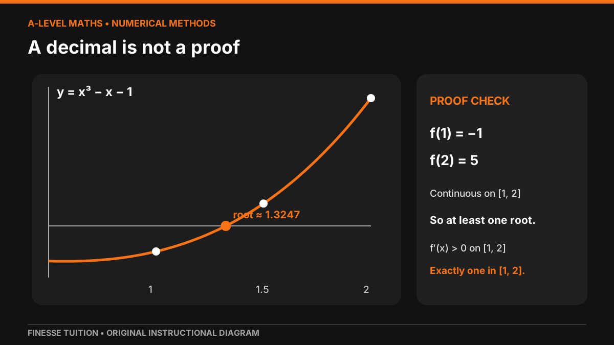
Let f(x)=x³−x−1. Begin by evaluating endpoints: f(1)=1−1−1=−1 and f(2)=8−2−1=5. The signs are opposite. Because f is a polynomial, it is continuous throughout [1,2]. The intermediate value theorem therefore guarantees at least one α between 1 and 2 for which f(α)=0. Write both numerical signs and the continuity statement explicitly.

Notice the phrase 'at least one'. A sign change does not normally prove uniqueness. For this particular function we can add an independent argument: f′(x)=3x²−1. For every x in [1,2], this derivative is positive, so the curve is strictly increasing in that interval and can cross the horizontal axis only once. We now know there is exactly one root in [1,2].

Make a habit of separating these statements: evidence of existence comes from continuity and opposite endpoint signs; evidence of uniqueness needs something else, such as a monotonicity argument. If you are under time pressure, a properly constructed sentence containing the correct interval is much more valuable than a long paragraph about what the graph seems to do.

• Evaluate the function at both stated endpoints, keeping its sign visible.
• Check that the function is continuous on the whole closed interval.
• State 'at least one root', not 'exactly one' unless you justify uniqueness separately.

Bisection: make the signs do the work

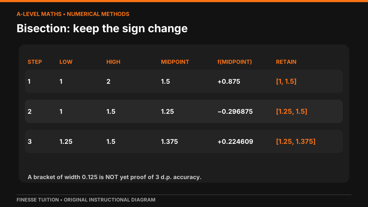
Now shrink the interval, retaining a sign change at every step. Start with [1,2]. The midpoint 1.5 gives f(1.5)=3.375−1.5−1=0.875. The negative value remains at x=1, so the new bracket is [1,1.5]. Repeating the midpoint test gives f(1.25)=1.953125−1.25−1=−0.296875, leaving [1.25,1.5]. The next midpoint is 1.375, where f(1.375)=0.224609375, so the bracket becomes [1.25,1.375].

Each midpoint halves the interval width and, for this continuous function, preserves a proven root within the new bracket. The third interval has width 0.125. It absolutely does not prove the solution is 1.325 to three decimal places. Keep iterating, or certify a sufficiently narrow interval by testing the required rounding boundaries. Precision must come from a bound, not from how many digits the display happens to show.

When you practise, write a brief reason for each retained half: 'left endpoint negative, midpoint positive, therefore root in the left half'. This is more transferable than memorising a particular calculator sequence. In an exam, keep at least enough working that the examiner can see which values determined each decision.

A sign change is a test with conditions

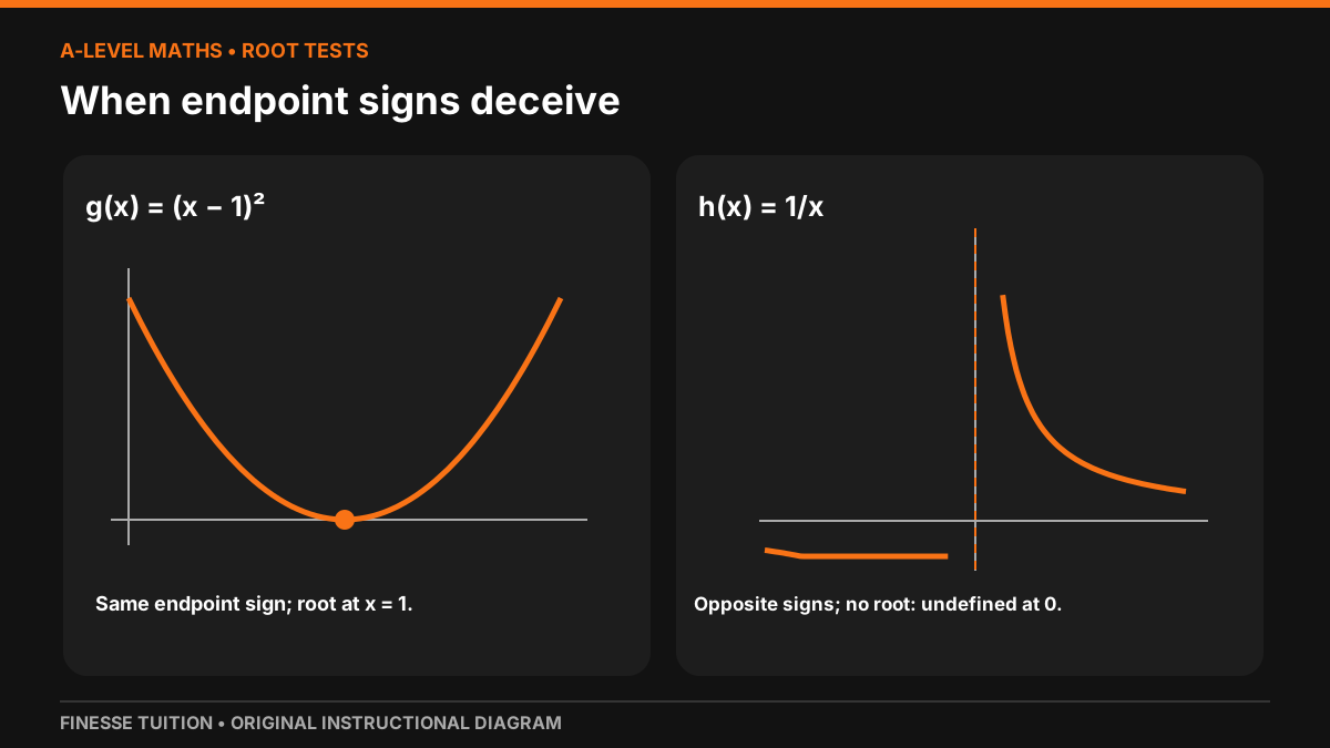
Here is why the continuity clause matters. Let g(x)=(x−1)² on [0,2]. Both endpoint values equal 1, so there is no sign change. Yet g(1)=0: the curve touches the axis before turning upwards again. Sign-change methods may miss repeated roots, so a failure to detect a sign change does not establish that there are no roots.

For a second counterexample, take h(x)=1/x on [−1,1]. We get h(−1)=−1 and h(1)=1. Those are opposite signs, but h has no root between −1 and 1 because the function is undefined at zero. It is not continuous on the entire interval. Opposite endpoint signs alone are insufficient; the intermediate value theorem is conditional.

These distinctions are useful whenever a question involves a rational expression, a graph with a break, or a repeated root. Before substituting numbers, check the domain and where the function is defined. Do not say 'no root' simply because the endpoint signs match, and never connect values across an asymptote as if the graph were continuous.

Iteration is a rule—not a lucky string of decimals

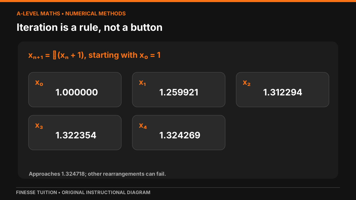
Rearrange x³−x−1=0 as x=∛(x+1). Define the recurrence xₙ₊₁=∛(xₙ+1), starting with x₀=1. Repeated substitution produces x₁≈1.259921, x₂≈1.312294, x₃≈1.322354, then values increasingly close to 1.324718. Write both the recurrence and its starting value: an unexplained table of answers is not a method somebody else could reproduce.

An iterative scheme is not guaranteed to converge merely because it is algebraically related to the original equation. Near a fixed point α, the size of g′(α) gives a useful local diagnostic: |g′(α)|<1 is associated with local attraction, subject to the conditions behind the test. For g(x)=∛(x+1), that magnitude is below one near the positive root. A different rearrangement can diverge or converge to another root.

Newton–Raphson uses tangent-line information: xₙ₊₁=xₙ−f(xₙ)/f′(xₙ). It can reach useful precision rapidly, but it may fail or behave badly if f′(xₙ) is zero or very small, or the initial estimate is poor. A confident A-Level student can both execute a recurrence and explain how its assumptions could break.

Approximate answers need accuracy certificates

The calculator value for our root is about 1.324717957. Rounding gives 1.325 to three decimal places, but if a question explicitly asks you to show that accuracy, construct the correct interval. A real number rounds to 1.325 to three decimal places if it lies between 1.3245 and 1.3255 under the usual rounding rule, with the upper boundary excluded.

For our continuous, strictly increasing f, a negative f(1.3245) and a positive f(1.3255) would establish that its single nearby root lies between those bounds. Check the arithmetic carefully rather than trusting signs from heavy early rounding. Alternatively, continue bisection until the entire retained root interval falls within the required rounding boundaries.

Do not confuse different numerical objectives. The trapezium rule approximates a definite integral by straight-line strips; it does not establish a root. An iteration supplies an approximate fixed point; it does not automatically prove the required number of decimal places. Precise working identifies the method, its target and the reason its result is credible.

Four easy ways to throw away a correct method

Your arithmetic can be immaculate and your mathematical conclusion incomplete. Look for four recurring categories rather than simply writing 'careless mistake' in your notebook. Recognition means deciding which result the question asks you to justify; condition checking means establishing the theorem's requirements; execution means evaluating or iterating accurately; interpretation means making the correct conclusion from those numbers.

Do not present these as quotations from an examiner report: they are a practical marking framework. Compare each answer against your own board's published guidance, including alternatives it accepts. Training the shape of the justification gives a better repair target than learning a phrase out of context. Correct reasoning, not a magic sentence, is what matters.

• Existence versus uniqueness: opposite signs plus continuity imply at least one root; uniqueness needs a further argument.
• Domain versus graph sketch: do not claim continuity across x=0 for 1/x.
• Approximation versus rounding proof: do not certify three decimal places from a bracket still 0.125 wide.
• Recurrence versus answer list: write the rule, starting value and reason to trust convergence.

The learning science: test the reason, not the screenshot

Once a worked example makes sense, close it. On blank paper, explain the intermediate value theorem in a sentence, identify one failure case, and carry out a sign-change test for a fresh function. Then check against an authoritative solution and immediately correct any wrong assumption. If you can only reproduce the exact original calculation, you have memorised a performance rather than built a transferable skill.

Roediger and Karpicke (2006) found that retrieval testing could improve retention on delayed tests compared with additional restudy in their experimental conditions. Dunlosky and colleagues (2013) assessed practice testing and distributed practice as broadly useful, while pointing to variation between settings and learning materials. These findings inform how we structure practice; they are not direct evidence that this exact numerical-methods routine raises A-Level grades by a specified amount.

Worked solutions are still essential at the start of a difficult technique, and timely feedback matters when your mental model is wrong. Use retrieval to diagnose whether you can execute and explain without prompts. If it reveals a misconception, return to a clear explanation, talk it through with a tutor if needed, then retest using a different function.

The 25-minute numerical-methods session

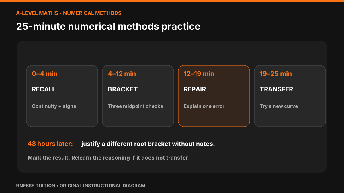
For minutes 0–4, recall the conditions for a root-existence argument and write one example of a misleading sign test. For minutes 4–12, take a new continuous function and run three labelled bisection steps. For minutes 12–19, compare the work with a checked solution and repair the most consequential error. For minutes 19–25, try a different function, explain which numerical method would be suitable and predict one risk of failure.

Return 48 hours later with no notes. Can you justify a bracket, recognise a discontinuity and describe why an iterative method might fail? Mark the result, revisit the relevant explanation, and test again using another unfamiliar example. Spacing is a flexible principle rather than a universal rule that every student needs the same exact delay.

Challenge yourself: find a continuous function with equal-sign endpoints but a root inside the interval, and a discontinuous function with opposite-sign endpoints but no root. If you can explain both, your understanding goes deeper than a calculator display.