Stop treating p-values like verdicts. Start interrogating the model.

The number can be right while the inference is wrong

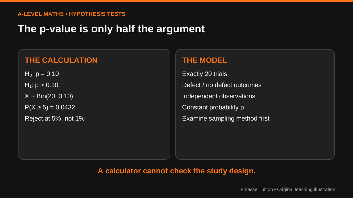
Here is an uncomfortable thought: the student who gets 0.0432 on a calculator can still deserve very few marks for the conclusion. A statistical test is an argument, not a button sequence. It starts with a claim about a population, makes assumptions about how observations arise, asks how surprising the sample would be if that claim were true, and then states a limited conclusion.

Many students learn hypothesis testing as a sequence of keystrokes. That approach appears to work until an unfamiliar exam question changes the setting. Suddenly they must decide whether the observations are independent, which tail to use, what the parameter means and how to describe the result without claiming proof. Those decisions are not optional extras: they are part of the mathematics.

This guide teaches a six-part audit that works for binomial tests in the AQA A-Level Mathematics 7357 specification. The same core concepts are encountered across English A-Level Mathematics boards, including Pearson Edexcel and OCR, though the exact paper structure and required notation should always be checked against your specification. The example data below are deliberately invented for teaching, not taken from an actual investigation.

First define p. Then write your hypotheses.

Imagine a manufacturer whose long-run proportion of defective components is thought to be 10%. A quality inspector suspects this proportion has increased. Define p to mean the probability that a randomly selected component from the production process is defective. Without that sentence, the symbol p floats free of the problem and your final conclusion risks describing the wrong population.

The null hypothesis is H₀: p = 0.10. The alternative is H₁: p > 0.10. The greater-than sign matters: it says the inspector is investigating an increase, so unusually HIGH numbers of defective items support the alternative. If the question instead asked whether the rate had fallen, H₁ would be p < 0.10 and the tail would change. If it asked whether the rate had changed in either direction, a two-tailed design would be needed.

Write the hypotheses before inspecting the sample whenever you can. Deciding on an increase only because the observed sample happened to be unusually high is a different procedure and can invalidate the claimed significance level. In an exam, the wording supplies the direction; outside the exam, decide it from the research question rather than the data you already saw.

Four assumptions are the real entrance exam

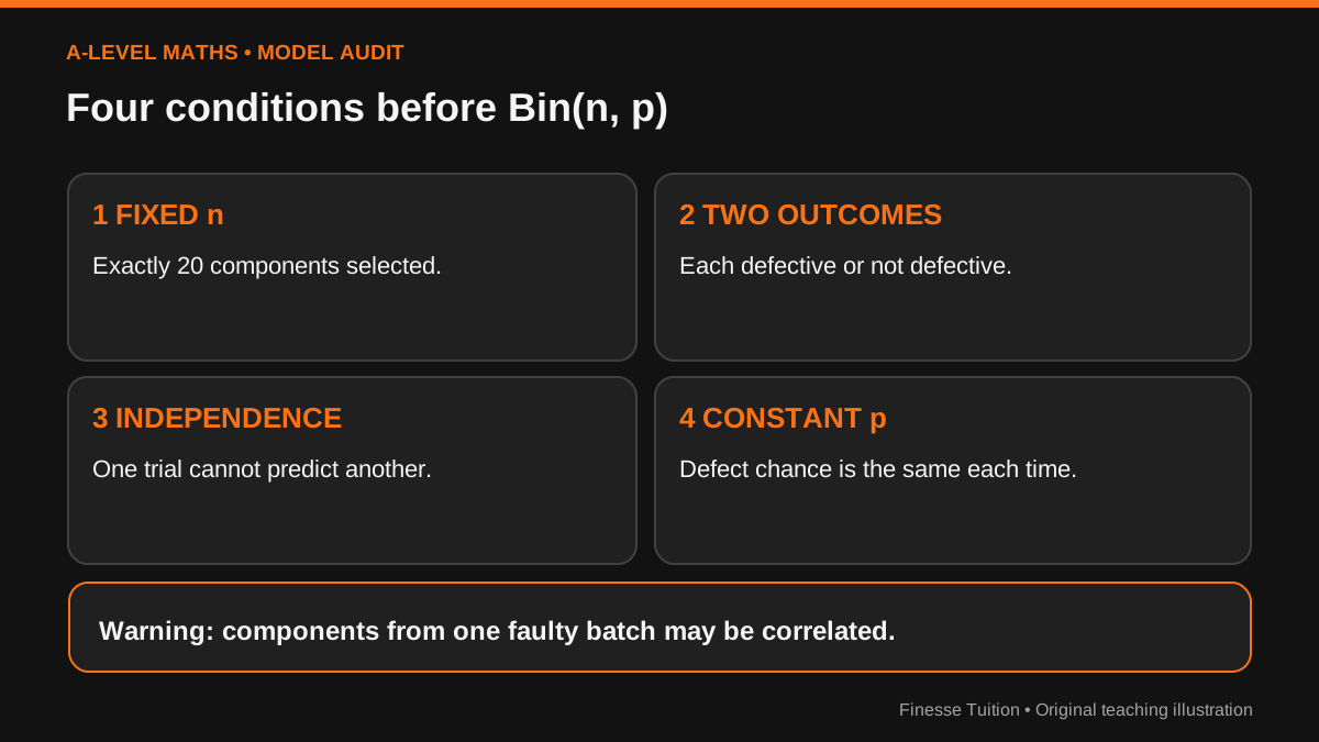
A binomial model is justified by fixed n, two outcomes on each trial, independence and a constant probability of the outcome of interest. Here the sample contains 20 components, each is classified defective or not, and the test assumes one component's status does not tell us about another's. Under the null, the probability of a defect on every trial is 0.10.

Independence is the assumption most likely to be invisible in a neat exam diagram. Twenty components taken consecutively from one malfunctioning machine could share a cause; a process that warms up over a shift could have a changing defect probability. Random sampling from a sufficiently large production run makes an independence approximation more plausible, but does not establish it automatically.

If those assumptions are unreasonable, calculating a binomial tail accurately does not rescue the model. Say exactly which assumption might fail and what information would help: sampling across different production times, inspecting whether the process was stable, or collecting data from independent batches. Do not confuse the accuracy of a calculator with the validity of the model.

Worked example: five defective items out of twenty

Suppose the inspector randomly selects 20 components under conditions where the assumptions are credible and finds five defective. Under H₀, let X be the number defective. Then X ~ Bin(20, 0.10). Because H₁ says the rate has increased, we need the probability of observing AT LEAST five defects if p really equals 0.10: P(X ≥ 5 | H₀).

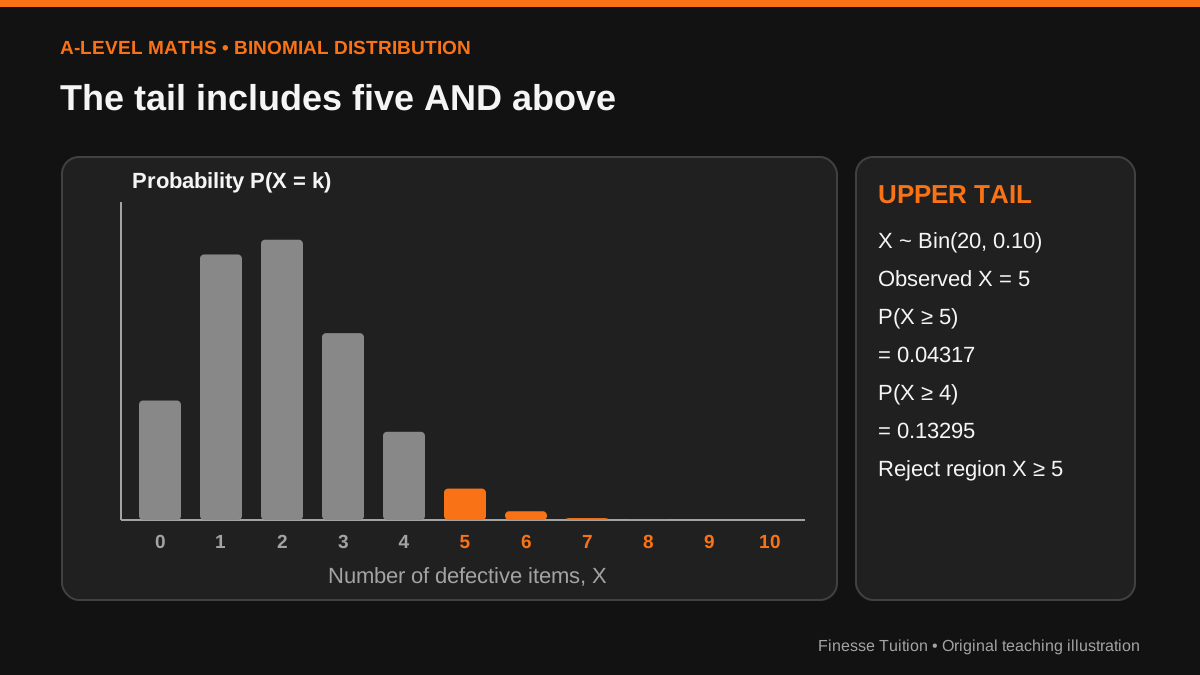
An exact binomial calculation gives P(X ≥ 5) = Σ from k = 5 to 20 of [20 choose k](0.10)^k(0.90)^(20−k) = 0.0431744953, approximately 0.0432. On a calculator, an equivalent route is 1 − P(X ≤ 4). Do not enter P(X = 5); that is only the probability of exactly five and leaves out outcomes six, seven and above.

The countercheck is useful: P(X ≥ 4) is approximately 0.13295. So at a 5% significance level, observing four defective components would not fall in the rejection region, but observing five would. The one-tailed 5% critical region is X ≥ 5. The bars above five are small, but they are still included in the p-value.

Reject at 5%. Not at 1%. Never claim you proved it.

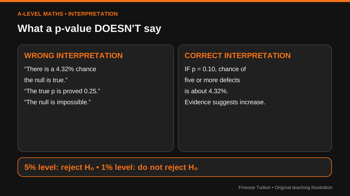
At the 5% level, 0.0432 < 0.05, so reject H₀. There is statistically significant evidence, under the binomial sampling assumptions, that the defective proportion has increased above 0.10. At the stricter 1% level, 0.0432 > 0.01, so there is insufficient evidence to reject H₀. The data and calculation did not change; the stated evidential threshold did.

The p-value is not the probability that H₀ is true. It is the probability, calculated assuming H₀, of an outcome at least as extreme in the direction of H₁. It also does not prove that the true defect probability is 25%, even though five out of twenty is a sample proportion of 0.25. A sample estimate and a conclusion about a population are different things.

At a nominal 5% significance level, a valid pre-specified testing procedure controls the long-run probability of wrongly rejecting a true null to at most about 5%; for this particular discrete upper-tail rejection rule under p = 0.10, the probability is approximately 4.32%. Neither number tells you the probability that your decision is wrong in this particular case.

The four interpretations that cost marks

Write the conclusion in the vocabulary of the original context. 'Reject H₀' is incomplete; the reader needs to know what the evidence concerns. 'Accept H₀' when you do not reject is also generally too strong. A non-significant result can reflect a small sample or weak evidence; it does not establish the null as fact.

Watch four common traps: choosing the lower tail for an increase; using the mass at exactly five instead of the whole upper tail; reporting P(H₀ is true) as 0.0432; and saying that the alternative has been proved. A fifth trap is choosing a one-tailed alternative after seeing the observed direction.

What the 2026 A-Level Maths results can—and cannot—show

Ofqual's 13 August 2026 overview reported that the proportion of Maths A-Level outcomes graded A* or A went from 41.6% in 2025 to 42.1% in 2026. That is a rise of 0.5 percentage POINTS, not a claim of 0.5% relative growth. Ofqual stated that the standard of work required for each Maths grade was unchanged and characterised the slightly higher top-grade proportion as reflecting a slightly stronger cohort.

Why put education news in a statistics lesson? Because one pair of percentages is not enough to establish a causal claim such as 'the papers were easier'. Differences in cohorts, assessment circumstances, populations and definitions matter. These are descriptive national results, not a binomial experiment with an agreed random-sampling model. Do not invent a p-value for them. This is the same intellectual discipline as checking the manufacturer example before running a test.

Practise the reasoning, not the calculator menu

Research on learning supplies a plausible reason to make students explain every step. Chi and colleagues (1994) found that prompted self-explanation supported deeper understanding in a small study involving younger learners reading about the circulatory system. Dunlosky and colleagues (2013) identified practice testing and distributed study as broadly useful strategies and rated self-explanation as promising with a more limited evidence base.

Those studies did not test this exact A-Level hypothesis-testing exercise or guarantee exam-grade improvements. The practical transfer is modest and testable: after each worked example, cover the solution and justify from memory what p means, why the model is binomial, why that tail was chosen, and what the decision can and cannot say. Then try a fresh question with a changed direction or changed context.

Keep a log of which part fails: model, hypotheses, tail, calculator operation or interpretation. Repair that specific step with feedback from the correct board mark scheme; do not spend twenty minutes repeating calculations you can already do reliably.

A 25-minute model-checking workout

Three short questions in different contexts are better diagnostic material than repeating one question until its numbers become familiar. The timings are a suggested training routine, not a scientifically validated optimum.

Return to one of the weaker steps after two or three days and again after about a week, using a new context. If you get it wrong, correct it with the worked answer immediately; unattended retrieval errors can become habits.

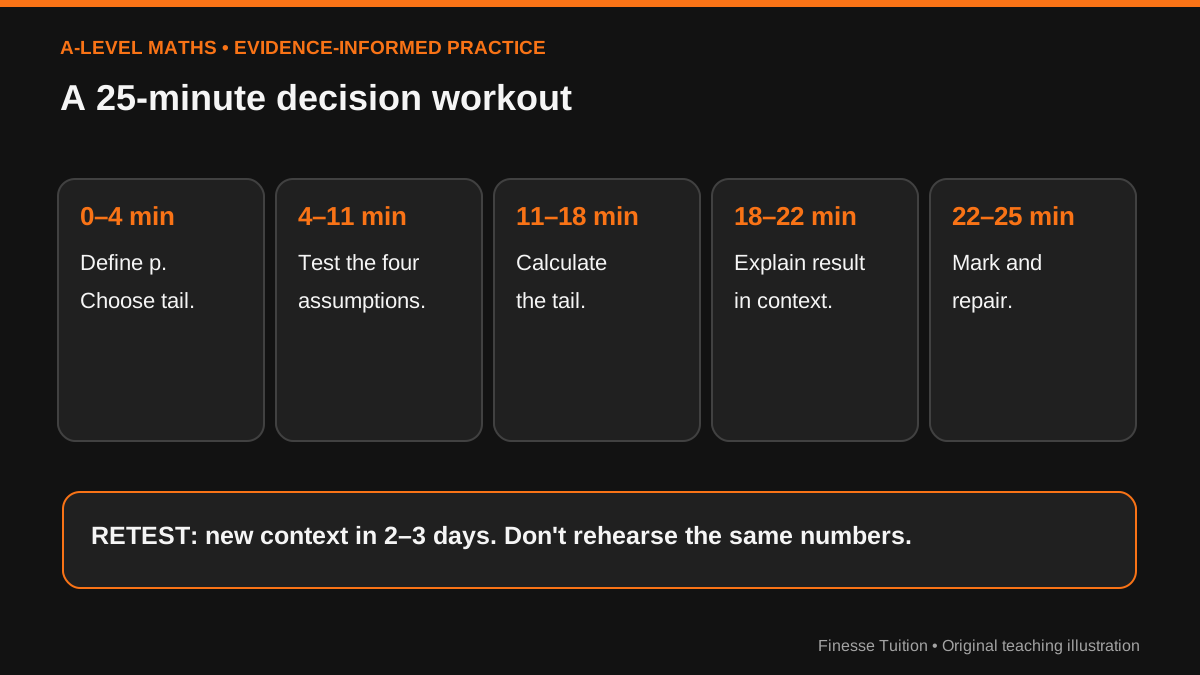
• 0–4 minutes: define the population parameter and identify which tail each research question implies.
• 4–11 minutes: check the four assumptions and set out H₀ and H₁ on an unseen question.
• 11–18 minutes: calculate a binomial tail, write a contextual decision and test the conclusion against a 1% threshold.
• 18–25 minutes: mark against an official scheme; correct the precise reasoning error and explain it from memory.
• Two or three days later: use a new context rather than memorising the old answer.

Where the evidence stops

Binomial tests are conditional models; they do not manufacture random assignment, remove confounding or prove causes. 'Statistically significant' describes a relationship between data, a model and a pre-specified threshold, not practical importance. Small effects can matter commercially; large-looking sample differences can also be inconclusive with limited data.

The routine above is an educational recommendation informed by general evidence about retrieval, spacing and metacognition, not a claim that one particular schedule raises A-Level results by a known percentage. Use it, measure errors on fresh timed tasks and adjust it as the exam approaches.