Part 2: Graphs, half-life and measuring rates

Learn which graph answers which question, then connect the plotted measurement to a defensible practical method.

Read the axes before deciding the order

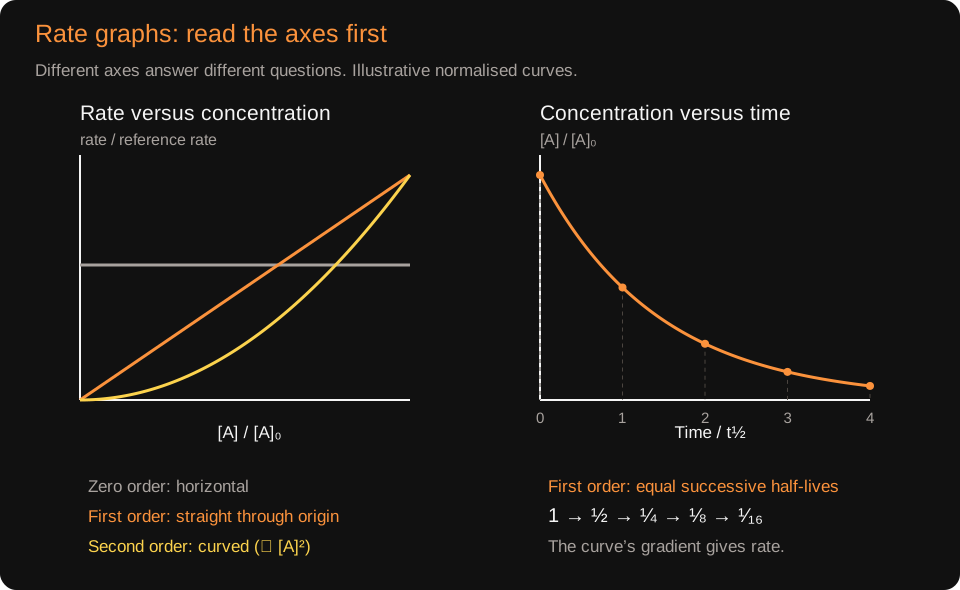
A concentration–time graph follows a single reaction mixture. Its gradient measures the rate at that moment; it is not itself a plot of rate against concentration. For a zero-order reactant, concentration falls linearly while the zero-order conditions hold. For a first-order reactant, the curve becomes less steep as concentration falls.

A rate–concentration graph compares measured rates at different concentrations with other relevant variables fixed. A horizontal line indicates zero order, a straight line through the origin first order and an upward quadratic curve second order. On a first-order rate–concentration graph the gradient is k because rate = k[A]. Do not apply that statement to a concentration–time graph.

Swipe horizontally to view the whole diagram.

Worked example: instantaneous rate is a tangent

Suppose a tangent at t = 40 s on an illustrative concentration–time curve passes through (20 s, 0.084 mol dm⁻³) and (70 s, 0.044 mol dm⁻³). Use those two well-separated points on the tangent, even though they need not both lie on the experimental curve.

Gradient = (0.044 − 0.084)/(70 − 20) = −8.0 × 10⁻⁴ mol dm⁻³ s⁻¹. The disappearance rate is 8.0 × 10⁻⁴ mol dm⁻³ s⁻¹. Drawing a line from the origin to the curve instead would generally give a mean over an interval, not the instantaneous rate at 40 s.

Why constant half-life identifies first order

Half-life is the time needed for a reactant concentration to fall to half its starting value for the interval considered. On a first-order curve, moving from 0.080 to 0.040, then 0.040 to 0.020 mol dm⁻³ takes equal time. The amount lost becomes smaller because the rate itself falls with concentration.

For an illustrative half-life of 120 s, k = ln 2/120 = 5.78 × 10⁻³ s⁻¹. After three half-lives, 1/8 of the initial concentration remains. A constant amount disappearing each minute instead suggests zero-order behaviour. OCR requires use of k = ln 2/t½, not derivation of an integrated rate law.

Continuous monitoring: choose a signal linked to concentration

A colorimeter can follow disappearance of a coloured reactant or formation of a coloured product. Choose a suitable filter or wavelength, zero with a solvent blank and use known standards to establish the relationship between absorbance and concentration. Keep the same clean cuvette orientation, path length and temperature; fingerprints and bubbles can alter light transmission.

Start timing at mixing and record readings at regular short intervals. Convert absorbance through the calibration relationship before plotting concentration against time unless proportionality has been established. A delay before the first reading can miss the steep initial region and underestimate an initial rate obtained from the recorded curve.

Alternative methods include gas volume or mass loss where the measured change can be related to the reacting amount. Apparatus must retain gas for a volume measurement, whereas a mass-loss setup deliberately lets the gas leave. Explain the link between the measured quantity and concentration; not every reaction has a useful colour or gas change. This develops PAG9/10 skills.

Initial-rate comparisons and clock reactions

Run separate mixtures with one concentration changed, constant total volume, fixed temperature and unchanged concentrations of other reactants. Replace omitted reagent volume with solvent where appropriate. Use c₁V₁/Vtotal to calculate the concentration after mixing; stock concentration is not automatically the reaction concentration.

A clock records the time to a fixed small extent of reaction, such as a colour endpoint produced after a fixed amount of scavenger is consumed. If the same small amount is required in every run, 1/t is proportional to the initial rate. It has units s⁻¹ and is not an absolute concentration rate unless multiplied by the fixed concentration change.

Repeat timings, use a consistent endpoint and keep the threshold small enough that reactant concentrations change little. A long clock time that consumes a substantial fraction of a reactant weakens the initial-rate approximation. Control temperature with a water bath and let solutions equilibrate before mixing, rather than merely recording room temperature.

Quick checks

Original Finesse questions. Reveal the indicative worked solutions after attempting each question; these are not official OCR A mark allocations.

Sources